Passion for CS

Hello Friends!!!
In this article, we are going to learn more methods of NumPy module. At the end of this article, you will be able to work on,

• ones
• zeros

So, let's start with these methods, these two methods are powerful as it is generally used to build feature vector with some default values while developing deep learning models.

• numpy.ones() - method returns an array with default value 1.0 with given shape or we can say newly returned array filled with 1.0 or 1 based on data type and shape.
• Syntax: numpy.ones(shape, dtype=None, order='C')
• Here, shape - is the shape of an array that you want to retrieve.
• dtype - is an optional argument, represents the data type of an array that you want to retrieve, the default data type is float.
• order{'C','F'} - is an optional argument, represents whether to store multi - dim array in C-style or Fortran style. C-style represents row-major and Fortran-style represents column-major in memory. 
• It returns ndarray object in the form of an array with the given shape, order and data type.

Let's move to another method.

• numpy.zeros() - method returns an array with default value 0.0, with given shape or we can say newly returned array filled with 0.0 or 0 based on data type and shape.
• Syntax: numpy.zeros(shape,dtype=float,order='C') 
• Here, shape - is the shape of an array that you want to retrieve.
• dtype - is an optional argument, represents the data type of an array that you want to retrieve, the default data type is float.
• order{'C','F'} - is an optional argument, represents whether to store multi - dim array in C-style or Fortran style. C-style represents row-major and Fortran-style represents column-major in memory. 
• It returns ndarray object in the form of an array with the given shape, order and data type.

Let's take an example of the above methods:

Helloooo Friends!!!

In the previous article, we have seen Bayes' theorem now we are going to learn Naive Bayes' classifiers.

• It is based on Bayes' theorem.
• It gives a strong predicted answer by applying Bayes' theorem. So, it is known as Naive Bayes' classifier.

Now, let's start with How does it work?

Let's take an example if we want to approve an application for a credit card, we need to check the age of a person, an income of a person, credit score, year of employment of a person, debts of a person, etc. Now we have two possibilities, approved or not approved. So, if we consider our outcomes as Res=1 if approved and Res=0 if not approved.

Add this problem to Bayes' equation so our problem with formula becomes something like:

Fig. 1 Whether to approve the application of credit card or not using Bayes' Theorem

Now we get the result Res=1 if the P(Res = 1 | x1,....,xn) > P(Res = 0 | x1,....,xn) otherwise Res=0.
P(Res = 1) is the prior probability, it works without knowing the values of x. (Here, x = {x1,x2,..., xn}).  So, that it works for P(Res = 0) + P(Res = 1) = 1. As we all know the total probability is 1. 
Next thing that we can to consider, P(Res | x1,....,xn) is class likelihood is the conditional probability that is Res has associated value of x.

And lastly, we have evidence or marginal probability is P(x1,....,xn) and is work when we consider the value of x, and we do not think whether the value of x is positive or negative.

Afterward, we can get the posterior probability is the combination of prior and result of Bayes' rule. So, as we have already discussed about that but again we think in the formula for our example with posterior probability is something like

Fig. 2 Posterior Probability

And Bayes' classifier chooses the result with the highest posterior probability from all the result. See the below formula for Bayes' classifier.

Fig. 3 Bayes' Classifier

So, in a simple meaning of Bayes' classifier, it is based on conditional probability and Bayes' rule, check for the posterior probability and choose the maximum or highest posterior probability to achieve the Classification task.

Now it is simple, isn't it? I hope you enjoy and learn this classifier easily.

Hello Friends!!!
Let's start again with NumPy module.
Today's methods for this module are mentioned below and at the end of this article, you will be able to manage numpy array with these methods.

• linspace
• empty

Linspace

Hello Friends!!!

Today in this article, we are going to learn about Naive Bayes Classifier, One more algorithm for classification. It is based on Bayes' theorem.
So, first of all, let's take a look at Bayes' theorem, this theorem is based on conditional probability.

What is Conditional Probability?

The probability which is assigned to an event A when it is known that another event B has occurred, or which would be assigned to A if it was known that B had occurred, which is known as "Conditional Probability" of A given to B. For example, the probability of getting raincoat in the market is connected with season.

Mathematical Definition of Conditional Probability

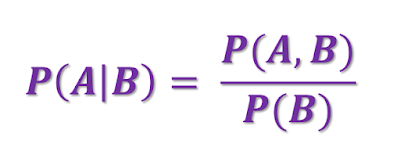
P(A|B) - represents the conditional probability of the event A given the event B; the probability assigned to A when it is known that the event B has occurred;
P(A,B) - represents the joint probability of event A and event B; i.e. the probability that both events A and B will occur.
(Resource: Probability and Statistics
for Business Decisions By Robert Schlaifer Professor of business administration Harvard University)

Now, we move to Bayes' theorem:

Bayes' theorem is used to describe the probability of an event based on some condition that may be related to an event. 

Fig. 2 Bayes' theorem equation

When we apply Bayes' theorem, it checks how the degree of beliefs, expressed as a probability.  It also accounting evidence.
 Let's understand the equation,
Here, P(A|B) represents a conditional probability, shows when the probability of an event A occurring given that event B is true.
same as with P(B|A) also a conditional probability, shows when the probability of an event B occurring given that event A is true.
P(A) and P(B) both are the probabilities of observing A and B independently and there is no relation with each other.

One more thing with this formula is: P(B) should not be 0.

For example,
In any medical test, such as Diabetes, the test is positive or negative. if the test is positive, detects diabetes otherwise not. we put this situation in the above equation.
P(A)=Diabetes detected
P(B)=Test is positive
P(B|A)=(Test = Positive | Diabetes = True)

P(A|B)=P(B|A)*P(A)/P(B)
P(Diabetes = True | Test = Positive)= P(Test = Positive | Diabetes = True)*P(Diabetes = True)  / P(Test = Positive)

That's it for this article in the next article we will learn Naive Bayes' theorem. I hope, you learn new things from this article...

Happy Learning....☺😊

Hello Friends!!! Welcome again,
Today we are going to discuss more methods of NumPy module. I hope you all do well with NumPy. So, let's start with NumPy and learn some more methods.

• numpy.delete - this method is used to remove elements from an array. it returns a new array with sub-array along with axis that is deleted.
• Syntax: numpy.delete(array,index,axis=None)
• Here, array - represents an array from which you want to remove elements.
• index - represents indexes of sub-arrays to remove along the specified axis. it may be any object.
• axis - is an optional parameter. represents an axis along which to delete the sub-array defined in an index argument. 
• It returns a ndarray. A copy of an array with the elements specified by the index removed.
• Example,

• numpy.concatenate - this method is used to join different arrays along with an existing axis.
• Syntax: numpy.concatenate((ar1, ar2, ...),axis=0,out=None)
• Here, ar1, ar2 - represents a sequence of arrays, all the array must have the same shape.
• axis - is an optional argument, represents axis along which arrays will be joined. here default value of this parameter is 0.
• out - is an optional parameter, it is ndarray object. represents the destination to place the result.
• It returns ndarray object after concatenation of arrays. 
• Example,  

These are methods of NumPy for this article that's it, in next article we will learn more methods.
Happy Learning & Coding...☺😊

Hello Friends!!!
This article takes some time, as I do work on some other articles also. Let's again work on NumPy, Kudos you all have learned some methods already from other articles of this module successfully. Now let's start with new methods with examples.

image (source: pixabay.com): Peoples are in a queue and new peoples are appended to the queue at the end of line

• numpy.append - This method is used to add (append)new values in an array at the end. 

• Syntax: numpy.append(array,values,axis=None)
• Here, array - is array-like values to be appended to the copy of the main array.
• values - is array-like values to be appended to the copy of the first argument array. it should be the same shape as the first argument has.
• axis - is an optional argument. it is used to set the axis on which array and values are to be appended.

• It returns ndarray object. copy array with values to the axis and append to ndarray.
• Example,
• It also gives ValueError, if axis of the array and values are different.