Passion for CS

Hello Friends,

Welcome to passionforcs!!!

In previous article, we have seen what is cost function? if you haven't checked please find to get the detail about the cost function and make it clear.

In this article, we are going to learn formula of cost function. How to calculate cost function?

Let's briefly revise once what is cost function? cost function is the function to check whether the model works well or not. To check whether the model performs well or not we have hypothesis, i.e. our prediction. Now the question is How to get hypothesis?

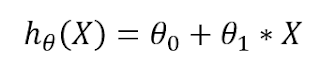
Now, you can get your prediction through the above equation. But here the question is what is theta (ϴ)?

So the answer is, ϴ is an additional parameter.

Now we have one more question, i.e. why? what is the need of the additional parameter?

Let me give you an example so you can get easily,

Consider our previous example, stock price prediction now we just analyze the stock or share price and make our prediction. We can set an input feature vector or simply consider one input feature only here, the input is opening price, closing price, high and low price etc. etc. but additional parameter that we need in this example is our money i.e. how much amount you want to invest? through which we can get how much profit or loss I will have? this investment is additional parameter we can say because it depends on us i.e. investor.

Now, let's consider the formula of cost function.

the above formula is the formula of cost function of linear regression. This is also known as squared error cost function.

Here, 1/2 * m -  m is number of samples in data or training set. 1/2 is used because when we take derivative of cost function to update the parameter during gradient descent at that time square (2 in the power) get cancelled with 1/2 multiplier thus derivation is cleaner.

Sigma (𝚺) - represents the sum.

h_ϴ(x⁽ⁱ⁾) - hypothesis prediction of input x at i^th index. (hypothesis value of h(x) if we use single value)

y⁽ⁱ⁾ - the actual label value for the input x at i^th index.

Just subtract actual value i.e. y from hypothesis prediction (predicted value) i.e. h(x) and square the achieved result.

This is just the calculation of cost function with MSE i.e. Mean Squared Error. We will learn more with example.

Till then try to get some cost by putting some values of x and theta.

Stay Safe Anywhere. :)

When we train our model, at that time also we should think about how our model performs? we can do this by using cost function to check whether our model performs well or not. Our hypothesis is valid and true so that the model gets the appropriate prediction or not.

In simple words the main usage of the cost function is after getting the prediction, how far or close our predicted values are from the actual values (i.e. label y).

Let's first prove these words by using the simple example.

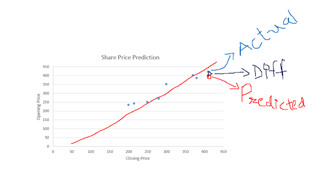
Suppose our model predict a price of a share A, So the price of the share A for today is around 410 this is the prediction and the actual value of the share A is 415 so the difference between the actual value and predicted value is 5, but if our predicted value is 450 and actual price is 400 of the share A then the difference between these two is 50.

When the difference is 5 we can say our model works fine for the share A, but when the difference is too high such as 50, our model doesn't predict well.

This is the cost function. When we build a model, we have to check the cost function to find whether our model performs well or not. A cost of a good model should be minimum.

So, through the above figure, we can get that blue dot is actual value, red square is predicted values and dark blue triangle is the difference but if difference is too big, the model doesn't predict well.

Hope you enjoy this article, Stay Home, Stay Safe.

Hello Friends!!!

This is the third algorithm, here I am going to share the support vector machine one more classification algorithm there are more classification algorithms I recommend you to refer these articles Logistic Regression and Naive Bayes classifiers to get proper ideas about classification algorithms.

SVM is really a very simple algorithm that works more accurately with less computational work. Actually, the support vector machine is a model works on a supervised learning technique, it works on both regression and classification. And generally suitable for binary classification. SVM is used to separate N - Dim hyperplane. For Example, if we have labeled data such as an image is a cat or not a cat. Here, we have two different labels Cat and Not and SVM Separates these labels on a hyperplane.

Fig. SVM Separates Labels

The above figure shows that the SVM separates the 2D hyperplane. In the above example, we have two labels blue dots represent Cat label and the orange triangle represents Not a Cat label. And in the above figure, one can see the separation of two different labels.

So, That's it you can get easily what is the meaning of Support Vector Machine? In the next article, we will learn more about SVM.

Hello Friends!!!
In this article, we are going to learn more methods of NumPy module. At the end of this article, you will be able to work on,

• ones
• zeros

So, let's start with these methods, these two methods are powerful as it is generally used to build feature vector with some default values while developing deep learning models.

• numpy.ones() - method returns an array with default value 1.0 with given shape or we can say newly returned array filled with 1.0 or 1 based on data type and shape.
• Syntax: numpy.ones(shape, dtype=None, order='C')
• Here, shape - is the shape of an array that you want to retrieve.
• dtype - is an optional argument, represents the data type of an array that you want to retrieve, the default data type is float.
• order{'C','F'} - is an optional argument, represents whether to store multi - dim array in C-style or Fortran style. C-style represents row-major and Fortran-style represents column-major in memory. 
• It returns ndarray object in the form of an array with the given shape, order and data type.

Let's move to another method.

• numpy.zeros() - method returns an array with default value 0.0, with given shape or we can say newly returned array filled with 0.0 or 0 based on data type and shape.
• Syntax: numpy.zeros(shape,dtype=float,order='C') 
• Here, shape - is the shape of an array that you want to retrieve.
• dtype - is an optional argument, represents the data type of an array that you want to retrieve, the default data type is float.
• order{'C','F'} - is an optional argument, represents whether to store multi - dim array in C-style or Fortran style. C-style represents row-major and Fortran-style represents column-major in memory. 
• It returns ndarray object in the form of an array with the given shape, order and data type.

Let's take an example of the above methods:

Helloooo Friends!!!

In the previous article, we have seen Bayes' theorem now we are going to learn Naive Bayes' classifiers.

• It is based on Bayes' theorem.
• It gives a strong predicted answer by applying Bayes' theorem. So, it is known as Naive Bayes' classifier.

Now, let's start with How does it work?

Let's take an example if we want to approve an application for a credit card, we need to check the age of a person, an income of a person, credit score, year of employment of a person, debts of a person, etc. Now we have two possibilities, approved or not approved. So, if we consider our outcomes as Res=1 if approved and Res=0 if not approved.

Add this problem to Bayes' equation so our problem with formula becomes something like:

Fig. 1 Whether to approve the application of credit card or not using Bayes' Theorem

Now we get the result Res=1 if the P(Res = 1 | x1,....,xn) > P(Res = 0 | x1,....,xn) otherwise Res=0.
P(Res = 1) is the prior probability, it works without knowing the values of x. (Here, x = {x1,x2,..., xn}).  So, that it works for P(Res = 0) + P(Res = 1) = 1. As we all know the total probability is 1. 
Next thing that we can to consider, P(Res | x1,....,xn) is class likelihood is the conditional probability that is Res has associated value of x.

And lastly, we have evidence or marginal probability is P(x1,....,xn) and is work when we consider the value of x, and we do not think whether the value of x is positive or negative.

Afterward, we can get the posterior probability is the combination of prior and result of Bayes' rule. So, as we have already discussed about that but again we think in the formula for our example with posterior probability is something like

Fig. 2 Posterior Probability

And Bayes' classifier chooses the result with the highest posterior probability from all the result. See the below formula for Bayes' classifier.

Fig. 3 Bayes' Classifier

So, in a simple meaning of Bayes' classifier, it is based on conditional probability and Bayes' rule, check for the posterior probability and choose the maximum or highest posterior probability to achieve the Classification task.

Now it is simple, isn't it? I hope you enjoy and learn this classifier easily.